11  Regression Models

---

Regression models are a fundamental part of supervised learning, used to predict continuous numerical values based on input variables. These models identify relationships between independent variables (features) and a dependent variable (target) to make predictions.

11.1 Regression Models

Regression is widely applied in fields such as finance, economics, healthcare, marketing, and agriculture for forecasting, trend analysis, and decision-making.

11.1.1 Summary of Regression Models

Model	Use Case	Advantages	Limitations
Linear Regression	House price prediction, salary estimation	Simple, easy to interpret	Assumes linearity, sensitive to outliers
Nonlinear Regression	Population growth, disease spread	Models complex relationships	Harder to interpret, computationally expensive
Multiple Regression	Predicting demand based on multiple factors	Captures multiple influences	Overfitting risk, requires careful variable selection
Polynomial Regression	Economic cycles, trajectory prediction	Fits curved trends	Overfitting with high-degree polynomials
Quantile Regression	Risk modeling, income distribution	Robust to outliers	Computationally intensive

Regression models form the backbone of predictive analytics, enabling accurate forecasting and decision-making in various domains, including business, healthcare, finance, and agriculture.

11.2 Linear Regression

Linear regression is the simplest and most commonly used regression model. It establishes a linear relationship between independent variables (X) and a dependent variable (Y) using a straight-line equation:

\[ Y = \beta_0 + \beta_1 X + \varepsilon \]

where:

• β₀ = Intercept (constant term)
• β₁ = Slope (coefficient)
• X = Independent variable
• ε = Error term (residual)

Example Applications

• Predicting house prices based on square footage and location.
• Forecasting sales revenue using advertising spend.
• Estimating employee salaries based on experience and education.

Advantages

• Easy to interpret and implement.
• Works well for data with a linear relationship.
• Computationally efficient.

Limitations

• Assumes a linear relationship, which may not always be the case.
• Sensitive to outliers.

11.2.1 Example: Linear Regression

Problem Statement

A real estate company wants to predict house prices based on square footage. The company collected a sample of 30 houses with their respective sizes (in square feet) and prices (in $1000s).

---

Sample Dataset

Below is the dataset containing 30 observations.

House Size (sq.ft)	Price ($1000s)
1500	300
1800	340
2100	400
2500	450
1300	260
1700	320
2200	420
2700	480
1600	310
1400	280
1900	360
2300	430
2800	490
2900	510
2000	370
2400	440
3000	520
2600	460
3100	530
3200	550
3300	570
3400	590
3500	610
3600	630
3700	650
3800	670
3900	690
4000	710
4100	730
4200	750

11.2.2 Performing Linear Regression in R

The linear regression model will be built using lm() function in R. The goal is to fit a model:

\[ \text{Price} = \beta_0 + \beta_1 \times \text{Size} \]

R Code Implementation

# Load necessary library
library(ggplot2)

# Sample dataset
house_data <- data.frame(
  Size = c(1500, 1800, 2100, 2500, 1300, 1700, 2200, 2700, 1600, 1400, 
           1900, 2300, 2800, 2900, 2000, 2400, 3000, 2600, 3100, 3200, 
           3300, 3400, 3500, 3600, 3700, 3800, 3900, 4000, 4100, 4200),
  Price = c(300, 340, 400, 450, 260, 320, 420, 480, 310, 280, 
            360, 430, 490, 510, 370, 440, 520, 460, 530, 550, 
            570, 590, 610, 630, 650, 670, 690, 710, 730, 750)
)

# Fit linear regression model
model <- lm(Price ~ Size, data = house_data)

# Summary of the model
summary(model)

Call:
lm(formula = Price ~ Size, data = house_data)

Residuals:
    Min      1Q  Median      3Q     Max 
-20.934  -7.801   1.000   8.098  20.129 

Coefficients:
             Estimate Std. Error t value Pr(>|t|)    
(Intercept) 46.658509   6.500969   7.177 8.23e-08 ***
Size         0.162670   0.002255  72.139  < 2e-16 ***
---
Signif. codes:  0 '***' 0.001 '**' 0.01 '*' 0.05 '.' 0.1 ' ' 1

Residual standard error: 10.69 on 28 degrees of freedom
Multiple R-squared:  0.9946,    Adjusted R-squared:  0.9945 
F-statistic:  5204 on 1 and 28 DF,  p-value: < 2.2e-16

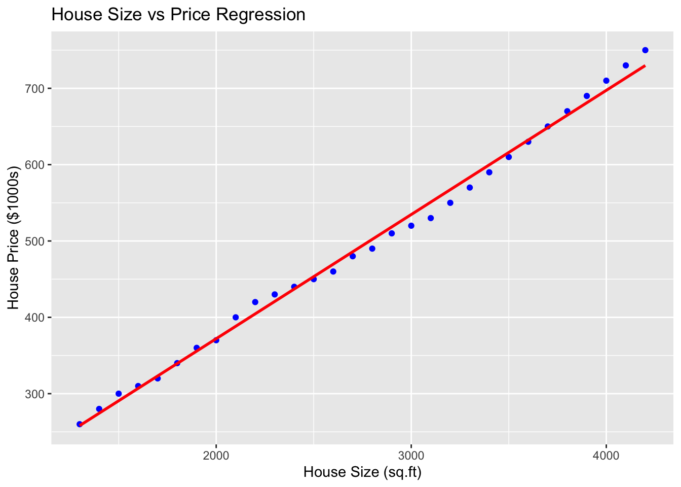
# Plot the data and regression line
ggplot(house_data, aes(x = Size, y = Price)) +
  geom_point(color = "blue") +
  geom_smooth(method = "lm", color = "red", se = FALSE) +
  labs(title = "House Size vs Price Regression",
       x = "House Size (sq.ft)",
       y = "House Price ($1000s)")

11.2.3 Interpretation of Results

R Output Explanation

• Intercept (\(\beta_0\) = 46.6585): Represents the baseline price when the house size is zero. Although a house with zero square footage is unrealistic, this value is necessary for the linear equation.
• Slope (\(\beta_1\) = 0.16267): Indicates that for each additional 1 sq.ft, the house price increases by $162.67.

The linear regression equation based on the output is:

\[ \text{Price} = 46.6585 + 0.16267 \times \text{Size} \]

Example Calculation

For a 2500 sq.ft house:

\[ \text{Price} = 46.6585 + (0.16267 \times 2500) \]

\[ = 46.6585 + 406.675 \]

\[ = 453.33 \]

Since the prices are in $1000s, the predicted price for a 2500 sq.ft house is $453,330.

Note:

• The intercept (\(\beta_0\) = 46.6585) is a mathematical reference point but may not have a direct real-world meaning.
• The slope (\(\beta_1\) = 0.16267) tells us that for every extra 1000 sq.ft, the price increases by approximately $162,670.
• This model allows us to estimate house prices based on size, assuming all other factors remain constant.
• You can use this equation to predict house prices for any given size.

---

11.2.4 Performing Linear Regression in Excel

Steps to Perform Regression in Excel

1. Enter the Data:
   • Open Excel and enter the Size in column A and Price in column B.
2. Using Data Analysis Tool:
   • Go to Data → Data Analysis → Regression.
   • Select Input Y Range (Price column).
   • Select Input X Range (Size column).
   • Click OK.
3. Interpret the Results:
   • Intercept (\(\beta_0\)): Represents the base price when size is 0.
   • Slope (\(\beta_1\)): Represents the increase in price per square foot.

---

11.2.5 Performing Linear Regression in SPSS

Load Data from Excel into SPSS

• Open SPSS.
• Click on File → Open → Data.
• Select Excel (.xls, .xlsx) as the file type and browse to your Excel file.
• Ensure the “Read variable names from the first row of data” option is checked.
• Click Open to import the data.

Run the Regression Analysis

• Click on Analyze → Regression → Linear.
• In the Linear Regression dialog box:
  • Move Price to the Dependent variable box.
  • Move Size to the Independent(s) variable box.
• Click OK to run the regression.

Interpret the Results

• Intercept (\(\beta_0\)): Represents the base price when the house size is zero.
• Slope (\(\beta_1\)): Represents the additional price per square foot.
• The R-squared value indicates how well the model explains the variation in house prices.
• The p-value for Size determines whether the relationship between size and price is statistically significant.

---

11.3 Multiple Regression

11.3.1 Overview

Multiple regression extends linear regression by incorporating multiple independent variables to predict a single dependent variable. The equation is:

\[ Y = \beta_0 + \beta_1X_1 + \beta_2X_2 + \dots + \beta_nX_n + \varepsilon \]

where:

• X₁, X₂, …, Xn are multiple independent variables.
• β₀, β₁, …, βn are coefficients.

Example Applications

• Predicting a car’s fuel efficiency based on weight, horsepower, and engine size.
• Estimating student performance based on study hours, attendance, and parental education.
• Forecasting demand for a product using advertising spend, economic indicators, and competitor pricing.

Advantages

• Captures multiple factors affecting the target variable.
• Provides a more comprehensive predictive model.

Limitations

• Higher complexity increases the risk of overfitting.
• Requires careful selection of variables to avoid multicollinearity.

---

11.4 Polynomial Regression

11.4.1 Overview

Polynomial regression extends linear regression by adding higher-degree polynomial terms to model curved relationships.

The equation is:

Y = β₀ + β₁X + β₂X² + β₃X³ + ... + βnX^n + ε

where:

• X², X³, …, Xⁿ are polynomial terms capturing the curvature in data.

Example Applications

• Predicting the trajectory of a projectile in physics.
• Modeling economic cycles where trends fluctuate over time.
• Fitting complex growth curves in biology and medicine.

Advantages

• Provides better accuracy than linear regression for non-linear data.
• Captures curved trends that linear models miss.

Limitations

• Prone to overfitting if the polynomial degree is too high.
• More complex than simple linear regression.

Example: Polynomial Regression

A real estate company wants to predict house prices based on square footage. The company believes that price does not increase linearly with size, but follows a non-linear pattern. To capture this relationship, they decide to use Polynomial Regression.

---

Sample Dataset

Below is a dataset containing 30 observations.

House Size (sq.ft)	Price ($1000s)
1500	300
1800	340
2100	400
2500	450
1300	260
1700	320
2200	420
2700	480
1600	310
1400	280
1900	360
2300	430
2800	490
2900	510
2000	370
2400	440
3000	520
2600	460
3100	530
3200	550
3300	570
3400	590
3500	610
3600	630
3700	650
3800	670
3900	690
4000	710
4100	730
4200	750

11.4.2 Performing Polynomial Regression in R

Polynomial regression is useful when linear models do not capture the pattern in the data.

R Code Implementation

# Load necessary library
library(ggplot2)

# Sample dataset (with a clear polynomial trend)
house_data <- data.frame(
  Size = c(1000, 1200, 1500, 1800, 2000, 2300, 2500, 2800, 3000, 3300, 
           3500, 3700, 4000, 4200, 4500, 4700, 5000, 5300, 5500, 5800),
  Price = c(100, 140, 200, 270, 350, 440, 500, 600, 700, 850, 
            950, 1100, 1250, 1400, 1600, 1800, 2050, 2300, 2500, 2800)
)

# Fit polynomial regression model (degree = 2)
model_poly <- lm(Price ~ poly(Size, 2, raw = TRUE), data = house_data)

# Generate fitted values
house_data$Predicted <- predict(model_poly)

# Summary of the model
summary(model_poly)

Call:
lm(formula = Price ~ poly(Size, 2, raw = TRUE), data = house_data)

Residuals:
    Min      1Q  Median      3Q     Max 
-32.951 -10.084   0.264  11.347  31.732 

Coefficients:
                             Estimate Std. Error t value Pr(>|t|)    
(Intercept)                 1.249e+02  2.255e+01   5.540 3.60e-05 ***
poly(Size, 2, raw = TRUE)1 -9.408e-02  1.473e-02  -6.387 6.76e-06 ***
poly(Size, 2, raw = TRUE)2  9.538e-05  2.136e-06  44.646  < 2e-16 ***
---
Signif. codes:  0 '***' 0.001 '**' 0.01 '*' 0.05 '.' 0.1 ' ' 1

Residual standard error: 18.22 on 17 degrees of freedom
Multiple R-squared:  0.9996,    Adjusted R-squared:  0.9995 
F-statistic: 2.005e+04 on 2 and 17 DF,  p-value: < 2.2e-16

# Plot the data and polynomial regression curve
ggplot(house_data, aes(x = Size, y = Price)) +
  geom_point(color = "blue", size = 3) +  # Scatter plot of actual data points
  geom_line(aes(y = Predicted), color = "red", size = 1.5) +  # Polynomial curve
  labs(title = "House Size vs Price (Polynomial Regression)",
       x = "House Size (sq.ft)",
       y = "House Price ($1000s)") +
  theme_minimal()

11.4.3 Interpretation of Results

R Output Explanation

The polynomial regression model captures the curved relationship between house size and price. The inclusion of a quadratic term ((^2)) allows the model to account for non-linearity in the data.

Regression Equation

The fitted polynomial regression equation from the R output is:

\[ \text{Price} = 124.9 - 0.094 \times \text{Size} + 9.538 \times 10^{-5} \times \text{Size}^2 \]

Interpretation of Coefficients

• Intercept (\(\beta_0 = 124.9\)): Represents the estimated base price when the house size is zero. While a size of zero is unrealistic, this value serves as a mathematical reference point.
  
• Linear Term (\(\beta_1 = -0.094\)): The first-degree coefficient suggests that, initially, as Size increases, the impact on Price is negative. However, this alone does not define the final trend since the quadratic term modifies the relationship.
  
• Quadratic Term (\(\beta_2 = 9.538 \times 10^{-5}\)): The positive second-degree term dominates for larger house sizes, creating a U-shaped relationship where Price first decreases slightly and then increases significantly as Size grows.

Example Calculation for a 2500 sq.ft House

Using the regression equation:

\[ \text{Price} = 124.9 + (-0.094 \times 2500) + (9.538 \times 10^{-5} \times 2500^2) \]

\[ = 124.9 - 235 + (9.538 \times 6,250,000) \]

\[ = 124.9 - 235 + 596.1 \]

\[ = 486 \]

Thus, the predicted house price for a 2500 sq.ft home is $486,000.

---

11.4.4 Performing Polynomial Regression in Excel

Steps to Perform Regression in Excel

1. Enter the Data:
   • Open Excel and enter the Size in column A and Price in column B.
2. Create Additional Columns for Polynomial Terms:
   • In column C, compute Size² using =A2^2.
3. Using Data Analysis Tool:
   • Go to Data → Data Analysis → Regression.
   • Select Input Y Range (Price column).
   • Select Input X Range (Size and Size² columns).
   • Click OK.
4. Interpret the Results:
   • Intercept (\(\beta_0\)): Represents the base price when size is 0.
   • Size Coefficient (\(\beta_1\)): Linear term.
   • Size² Coefficient (\(\beta_2\)): Captures non-linearity.

---

11.4.5 Performing Polynomial Regression in SPSS

Load Data from Excel into SPSS

• Open SPSS.
• Click on File → Open → Data.
• Select Excel (.xls, .xlsx) as the file type and browse to your Excel file.
• Ensure the “Read variable names from the first row of data” option is checked.
• Click Open to import the data.

Run the Regression Analysis

• Click on Analyze → Regression → Linear.
• In the Linear Regression dialog box:
  • Move Price to the Dependent variable box.
  • Move Size and Size² to the Independent(s) variable box.
• Click OK to run the regression.

Interpret the Results

• Intercept (\(\beta_0\)): Represents the base price.
• Size (\(\beta_1\)): Linear effect.
• Size² (\(\beta_2\)): Captures non-linearity in house prices.

---

11.5 Nonlinear Regression

11.5.1 Overview

Nonlinear regression is used when the relationship between X and Y is not linear. It models complex patterns using curved functions such as exponential, logarithmic, and power functions.

Common nonlinear regression equations:

• Exponential: Y = a * e^(bX)
• Logarithmic: Y = a + b * log(X)
• Power: Y = a * X^b

Example Applications

• Modeling population growth using an exponential function.
• Predicting disease spread in epidemiology.
• Analyzing chemical reaction rates in physics and chemistry.

Advantages

• Can model more complex relationships than linear regression.
• Provides better accuracy when data is not linearly distributed.

Limitations

• More complex to interpret and implement.
• Requires more computational power.

---

11.6 Quantile Regression

11.6.1 Overview

Quantile regression estimates conditional quantiles of the dependent variable instead of just predicting the mean (as in linear regression). This makes it more robust to outliers and useful for heterogeneous distributions.

Instead of:

Y = β₀ + β₁X + ε

Quantile regression models different quantiles (e.g., 25th, 50th, 75th percentiles) by minimizing an asymmetric loss function.

Example Applications

• House price estimation for different market segments (luxury, mid-range, affordable).
• Income distribution modeling across various economic groups.
• Risk assessment in finance by predicting high-loss scenarios.

Advantages

• More robust to outliers than standard linear regression.
• Suitable for modeling skewed and heterogeneous data.

Limitations

• Computationally more complex.
• Harder to interpret compared to standard linear regression.

---