3 Fundamentals of R and R Studio

3.1 Introduction to R programming

What is R ?

R, is a powerful language and environment for statistical computing and graphics.
R is an open-source programming language, widely used among statisticians, data analysts, and researchers for data manipulation, calculation, and graphical display.
R is not just a programming language, but also an environment for interactive statistical analysis.
It was developed by Ross Ihaka and Robert Gentleman at the University of Auckland, New Zealand, and is currently maintained by the R Development Core Team.
It is a GNU project and is freely available under the GNU General Public License.
Packages: The R community is known for its active contributions in terms of packages. There are thousands of packages available in the Comprehensive R Archive Network (CRAN), covering various functions and applications.
Platform Independent: R is available for various platforms such as Windows, MacOS, and Unix-like systems.

3.1.1 Installation and Setup

Install R

Download and install R from the Comprehensive R Archive Network (CRAN) and choose the relevant OS (Windows,mac,linux).

Install RStudio

RStudio is a recommended integrated development environment (IDE) for R. Download and install RStudio form POSIT and choose the relevant OS (Windows,mac,linux).

3.2 Basics of R Studio interface

3.2.1 Overview of RStudio Panels

RStudio is a widely-used Integrated Development Environment (IDE) for R programming.
RStudio’s design enhances the efficiency and user-friendliness of coding, testing, and data analysis in R.
Its panels and features provide a comprehensive environment that caters to the needs of both novice and experienced R programmers.
It features a user-friendly interface and is divided into several panels, each designed for specific tasks. Here’s a detailed overview of these panels.

Source Panel (Top-Left by Default)

Function

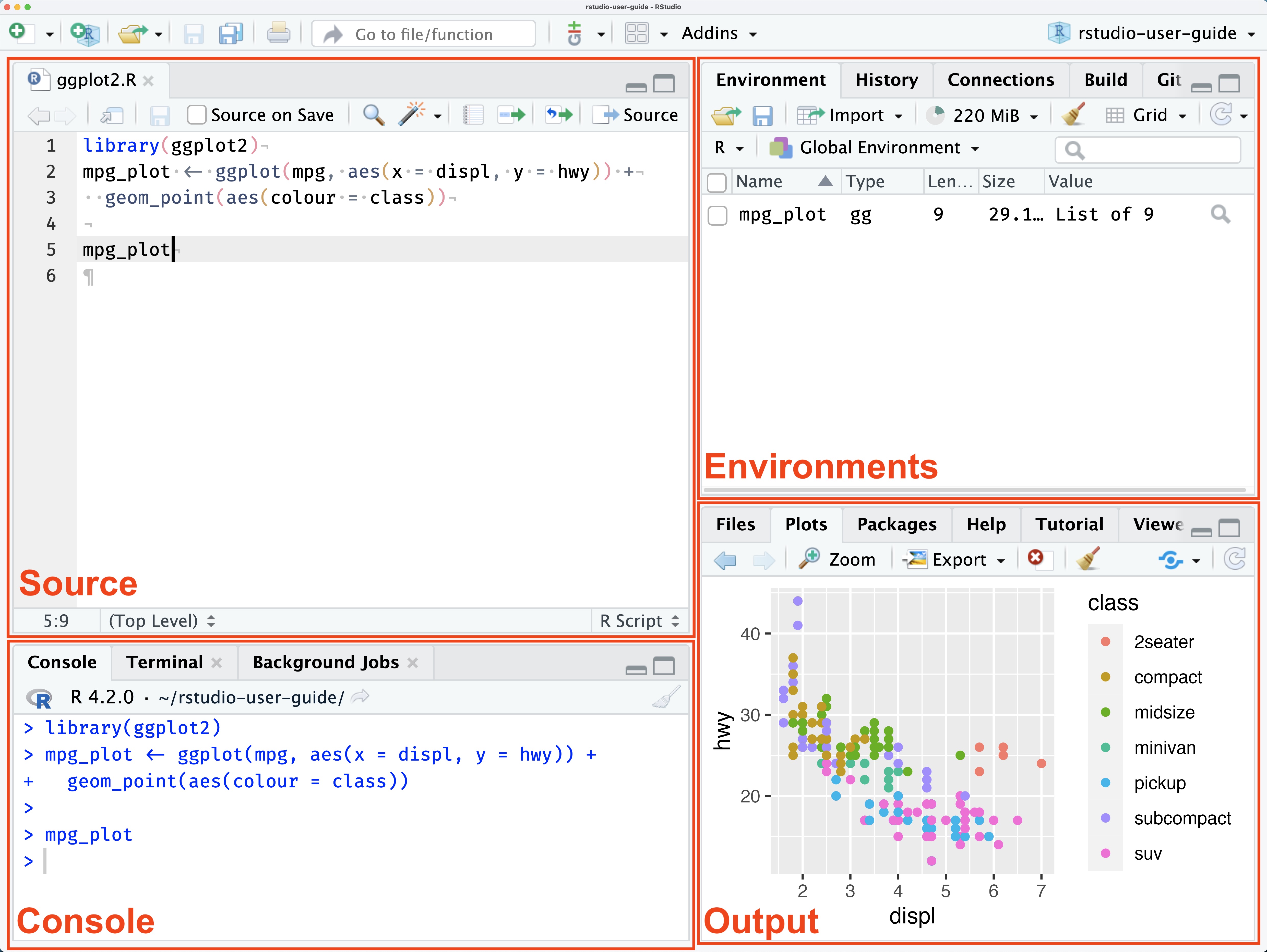
This panel is where you write and edit your R scripts and R Markdown documents.

Features

Syntax highlighting for R code.
Code completion and hinting.
Ability to run code directly from the script.

Console Panel (Bottom-Left by Default)

Function

This is where R code is executed interactively.

Features

Direct execution of R commands.
Displays results of script execution.
Keeps a history of your commands.

Environment/History Panel (Top-Right by Default)

Environment Tab

Shows the current working dataset and variables in memory.
Allows for inspection and management of data structures and variables.

History Tab

Records all commands run in the Console.
Enables re-running and insertion of previous commands into scripts.

Output/ Files/ Plots/ Packages/ Help/ Viewer Panel (Bottom-Right by Default)

Files Tab

Manages project files and directories.
Sets the working directory.

Plots Tab

Displays graphs and charts.
Allows for the export of plots.

Packages Tab

Lists and manages R packages.
Provides access to package documentation.

Help Tab

Offers R documentation and help files.
Useful for learning about R functions and packages.

Viewer Tab

Displays local web content such as HTML files from R Markdown or Shiny apps.

Additional Features

Toolbar: Quick access to common tasks like saving, loading, and running scripts.
Customization: Ability to rearrange the layout of tabs and panes.
Version Control: Integrated support for Git and SVN.

3.3 Fundamentals of R programming

3.3.1 R Syntax

R is a powerful programming language used extensively for statistical computing and graphics. It provides a wide array of techniques for data analysis, including linear and nonlinear modeling, classical statistical tests, time-series analysis, classification, clustering, and more. Its syntax allows users to easily manipulate data, perform calculations, and create graphical displays. Here’s a breakdown of some fundamental aspects of R syntax and an example to illustrate how it works.

Basic Syntax Components

Variables: In R, you can create variables without declaring their data type. You simply assign values directly with the assignment operator <- or =.
Comments: Comments start with the # symbol. Everything to the right of the # in a line is ignored by the interpreter.
Vectors: One of the basic data types in R is the vector, which you create using the c() function. Vectors are sequences of elements of the same type.
Functions: Functions are defined using the function keyword. They can take inputs (arguments), perform actions, and return a result.
Conditional Statements: R supports the usual if-else conditional constructs.
Loops: For iterating over sequences, R provides for, while, and repeat loops.
Packages: R’s functionality is extended through packages, which are collections of functions, data, and compiled code. You can install packages using the install.packages() function and load them with library().

3.3.2 R Script

Rscript is a tool for executing R scripts directly from the command line, making it easier to integrate R into automated processes or workflows.
It’s part of the R software environment, which is widely used for statistical computing and graphics. Rscript enables you to run R code saved in script files (typically with the .R extension) without opening an interactive R session.
This is particularly useful for batch processing, automated analyses, or running scripts on servers where a graphical user interface is not available.

Creating an R Script in RStudio

Creating and using R scripts in RStudio is a fundamental skill for anyone working with data in R. RStudio, being a powerful IDE for R, streamlines the process of writing, running, and managing R scripts. Here’s a concise guide based on insights from various sources:

Start a New Script: To begin, navigate to File -> New File -> R Script. This opens a new script tab in the top-left pane where you can write your code.
Writing Code: You can type your R code directly into this script pane. Common tasks include importing data, data manipulation, statistical analysis, and plotting. For instance, to create and print a variable, simply type something like result <- 3 followed by print(result) to see the output in the Console pane.
Running Code: To execute your code, you can click the Run button at the top of the script pane, or use keyboard shortcuts (e.g., Ctrl+Enter on Windows or Cmnd+Enter on Mac). The output will appear in the Console pane at the bottom.

Basic R Scripts Examples

Below are a few examples of basic R scripts that demonstrate common tasks in R.

Example 1: Hello World

A simple script that prints “Hello, World!” to the console.

Code

# Print "Hello, World!" to the console
print("Hello, World!")

[1] "Hello, World!"

Example 2: Basic Arithmetic

This script performs basic arithmetic operations and prints the results.

Code

# Perform arithmetic operations
add <- 5 + 3

# Print the results
add

[1] 8

Sample Rscript file

3.3.3 Data Types in R

Data types refer to the kind of data that can be stored and manipulated within a program. In R, the basic data types include:

Numeric: Represents real numbers (e.g., 2, 15.5).
Integer: Represents whole numbers (e.g., 2L, where L denotes an integer).
Character: Represents strings (e.g., “hello”, “1234”). Character must be put between “.
Logical: Represents Boolean values (TRUE or FALSE).

3.3.4 Basic Operators

Assignment Operator

The assignment operator in R is used to assign values to variables or objects in the R programming language.
The leftwards assignment operator <-: This is the most commonly used assignment operator in R. It assigns the value on its right to the object on its left. For example, x <- 3 assigns the value 3 to the variable x.
Alternative Assignment Operator (=) Apart from <-, R also supports the use of the = operator for assignments, similar to many other programming languages.
However, the use of <- is preferred in R for historical and readability reasons. For example, x = 3 is valid but x <- 3 is more idiomatic to R.

Use <- or = for assigning values, e.g., x <- 10 or x= 10

Code

x=5
x

[1] 5

Code

y <- 3
y

[1] 3

Commenting Code for Clarity

Use # for comments, e.g., # This is a comment.

Comments are not executable and are used to provide relevant information about the syntax. Whatever is typed after # symbol, is considered as comment.

Code

# Assigning values to x
x=5
x

[1] 5

Arithmetic operators

In R, arithmetic operators are used to perform common mathematical operations on numbers, vectors, matrices, and arrays. Here’s an overview of the primary arithmetic operators available in R: +, -, *, /, ^

Code

# Perform arithmetic operations
add <- 5 + 3

# Print the results
add

[1] 8

Division (/) operator - Divides the first number or vector by the second, element-wise.

Code

x=5
y=3
x/y

[1] 1.666667

Square (^) operator - Squares the first number by the second.

Code

x=5
x^2

[1] 25

3.3.5 Statements

Logical Operations

Includes ==, !=, >, <, >=, <=.

Equality: == checks if two values are equal.

Code

# Equality 5 == 3
x <- 5
y <- 3
x == y

[1] FALSE

Inequality: != checks if two values are not equal.

Code

# Inequality 5 != 3
x != y

[1] TRUE

Greater than: > checks if the value on the left is greater than the value on the right.

Code

# Greater than 5 > 3
x > y

[1] TRUE

Less than: < checks if the value on the left is less than the value on the right.

Code

# Less than 5 < 3
x < y

[1] FALSE

Greater than or equal to: >= checks if the value on the left is greater than or equal to the value on the right.

Code

# Greater than or equal to 5 >= 3
x >= y

[1] TRUE

Less than or equal to: <= checks if the value on the left is less than or equal to the value on the right.

Code

# Less than or equal to 5 <= 3
y <= x

[1] TRUE

3.3.6 Data Structures

Vectors

Vectors are fundamental data structures that hold elements of the same type.
They are one-dimensional arrays that can store numeric, character, or logical data.
Assigning data to vectors in R is a basic operation, essential for data manipulation and analysis.
The c() function combines values into a vector. It’s the most common method for creating vectors.

Code

creating vector

# Numeric vector
age <- c(20, 21, 23)
age

[1] 20 21 23

Code

# Character vector
student <- c("ajay", "vijay", "jay")
student

[1] "ajay"  "vijay" "jay"

Code

# logical vector
Pass<- c(TRUE, FALSE, TRUE) 
Pass

[1]  TRUE FALSE  TRUE

Matrix

A two-dimensional, rectangular collection of elements of the same type.
All elements must be of the same data type.
Created using the matrix() function. nrow is used to set number of rows and byrow is used to set values by rows (if TRUE) or columns (if FALSE).

Code

# Create a matrix with 2 rows and 3 columns
my_matrix <- matrix(data = c(1, 2, 3, 4, 5, 6), nrow = 2, ncol = 3, byrow = TRUE)

# Print the matrix
print(my_matrix)

     [,1] [,2] [,3]
[1,]    1    2    3
[2,]    4    5    6

Array

Similar to matrices but can have more than two dimensions.
Elements within an array must all be of the same data type.
Created using the array() function. dimensions are set using dim.

Code

# Create a 3-dimensional array with dimensions 2x3x2
my_array <- array(data = c(1:24), dim = c(2, 3, 4))

# Print the array
print(my_array)

, , 1

     [,1] [,2] [,3]
[1,]    1    3    5
[2,]    2    4    6

, , 2

     [,1] [,2] [,3]
[1,]    7    9   11
[2,]    8   10   12

, , 3

     [,1] [,2] [,3]
[1,]   13   15   17
[2,]   14   16   18

, , 4

     [,1] [,2] [,3]
[1,]   19   21   23
[2,]   20   22   24

3.3.7 Functions

Consists inbuilt functions like sum(), length(), sqrt(),mean(), summary(), View()

sum() Function

The sum() function calculates the total sum of all the elements in a numeric vector.

Code

sum function

# Calculate the sum of two variables
x=5
y=3
z=2
sum(x,y,z)

[1] 10

Code

# Calculate the sum of a numeric vector
numbers <- c(1, 2, 3)
sum(numbers)

[1] 6

length() Function

The length() function returns the number of elements in a vector (or other objects).

Code

length function

# Find the length of a vector
numbers <- c(1, 2, 3, 4, 5)
length(numbers)

[1] 5

sqrt() Function

The sqrt() function calculates the square root of each element in a numeric vector.

Code

square root function

# Calculate square root of a variable
x=25
sqrt(x)

[1] 5

Code

# Calculate the square root of each element in a numeric vector
numbers <- c(1, 4, 9, 16, 25)
sqrt(numbers)

[1] 1 2 3 4 5

mean() Function

The mean() function calculates the arithmetic mean (average) of the elements in a numeric vector.

Code

mean function

# Example: Calculate the mean of a numeric vector
numbers <- c(2,4,6)
mean(numbers)

[1] 4

summary() function

The summary() function in R provides a concise statistical summary of objects like vectors, matrices, data frames, and results of model fitting.

Code

summary function

# Create a numeric vector
vec <- c(1, 2, 3, 4, 5, NA, 7, 8, 9, 10)

# Get summary of the vector
summary(vec)

   Min. 1st Qu.  Median    Mean 3rd Qu.    Max.    NA's 
  1.000   3.000   5.000   5.444   8.000  10.000       1

data.frame() function

data.frame() function is used to create data frames, which are table-like structures consisting of rows and columns. - Data frames are one of the most important data structures in R, especially for statistical modeling and data analysis.

Code

creating data frame

# Creating a simple data frame
students <- data.frame(
  Name = c("Arun", "Bhavana", "Charan", "Divya", "Eswar", 
           "Fathima", "Gopal", "Harini", "Ilango", "Jayanthi"),
  Age = c(25, 30, 35, 28, 22, 40, 33, 27, 31, 29),
  Height = c(5.6, 5.5, 5.8, 5.4, 6.0, 5.3, 5.9, 5.5, 5.7, 5.8)
)
students

       Name Age Height
1      Arun  25    5.6
2   Bhavana  30    5.5
3    Charan  35    5.8
4     Divya  28    5.4
5     Eswar  22    6.0
6   Fathima  40    5.3
7     Gopal  33    5.9
8    Harini  27    5.5
9    Ilango  31    5.7
10 Jayanthi  29    5.8

head() function

The head() function in R is used to display the first few rows of a dataset, making it a useful tool for quickly inspecting large data frames or matrices.

Code

creating data frame

head(students)

     Name Age Height
1    Arun  25    5.6
2 Bhavana  30    5.5
3  Charan  35    5.8
4   Divya  28    5.4
5   Eswar  22    6.0
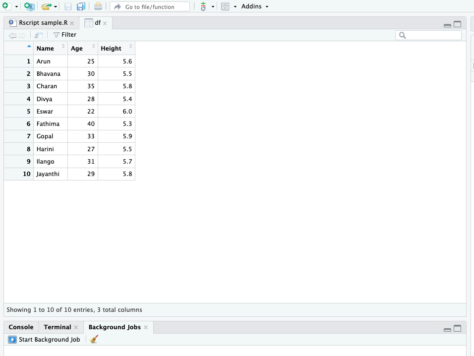
6 Fathima  40    5.3

View() function

View() function is used to invoke a spreadsheet-like data viewer on a data frame, matrix, or other objects that can be coerced into a data frame. - This function is particularly useful during interactive sessions to inspect data visually.

Code

View() function

# View function to see the data in a dedicated window
View(students)

3.3.8 Loops

Use for, while.

for loop

The for loop in R is used to iterate over a sequence (like a vector or a list) and execute a block of code for each element in the sequence.

Code

for loop

# Print numbers from 1 to 5
for(i in 1:5) {
  print(i)
}

[1] 1
[1] 2
[1] 3
[1] 4
[1] 5

while loop

The while loop executes a block of code as long as the specified condition is TRUE

Code

while loop

# Print numbers from 1 to 5 using while
i <- 1  # Initialize counter
while(i <= 4) {
  print(i)
  i <- i + 1  # Increment counte
}

[1] 1
[1] 2
[1] 3
[1] 4

3.4 R Markdown

3.4.1 Introduction to R Markdown

R Markdown is a powerful tool for integrating data analysis with documentation, allowing you to create dynamic reports and presentations.
It combines the core syntax of Markdown (a simple markup language for formatting text) with embedded R code chunks.
R Markdown documents are fully reproducible and support a wide range of output formats like HTML, PDF, and Word documents.

Key Features of R Markdown

Reproducible Research: Allows you to integrate your R code with your report, ensuring that your analysis can be easily reproduced.
Multiple Output Formats: You can convert a single R Markdown file into a variety of formats, including HTML, PDF, and Word.
Dynamic Content: Your document automatically updates its results whenever the underlying R code changes.
Integration with RStudio: R Markdown is tightly integrated with RStudio, making it easy to write, preview, and compile your document.

3.4.2 Creating an R Markdown File

In RStudio, you can create a new R Markdown file via the menu: File -> New File -> R Markdown....

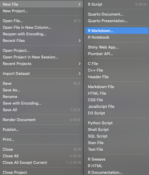This opens a dialog where you can choose the output format and other options.

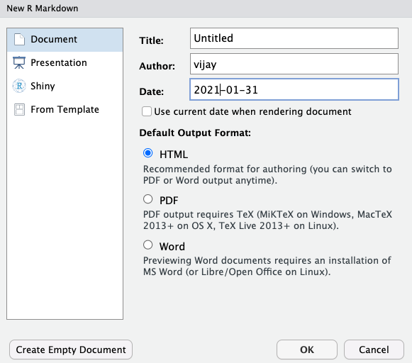Enter a title, author and date, check html for html output and click ok.

New R Markdown will open in a new window as shown below.

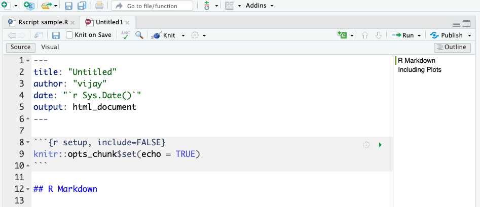
Default R Markdown Template in RStudio

When you create a new R Markdown file in RStudio, a default template is generated with the following components:

YAML Metadata (Document Header)

At the top of the document, you will see a YAML metadata block, enclosed within triple dashes ---. This section specifies document settings such as the title, author, date, and output format.
---
title: “Untitled”
author: “vijay”
date: “2025-04-18”
output: html_document
---

Setup Code Chunk

Immediately following the YAML header, a setup chunk is included:

{r setup, include=FALSE}

knitr::opts_chunk$set(echo = TRUE)

Purpose: This chunk sets options for how R code should be displayed and executed in the document.
knitr::opts_chunk$set(echo = TRUE): Ensures that R code is displayed along with its output.
include=FALSE: Hides this setup chunk from appearing in the final document.

Default Heading: “R Markdown”

# R Markdown

This is a section heading that introduces the user to R Markdown. It is placed there to provide a structured template for writing content.

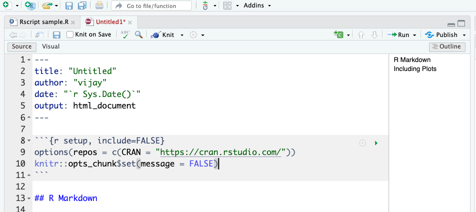
Insert the following code inside the r setup chunk.

options(repos = c(CRAN = "https://cran.rstudio.com/"))
knitr::opts_chunk$set(message = FALSE)

Including this code at the beginning of an RMarkdown file ensures that R uses a specific CRAN repository (https://cran.rstudio.com/) for package installation and suppresses unnecessary messages in code chunks, making the document cleaner and more readable.

It should look like the below.

Save the file with a file name

Compiling the Document: knit

After saving the file, compile the document into your desired output format. click the Knit button in RStudio. This will execute all R code within the document and render it to the specified output format.

3.4.3 Markdown Syntax

R Markdown supports standard Markdown syntax. Here are some basic examples:

Headers: Use # for headers. E.g., # Header 1, ## Header 2.
Bold and Italic: Use **bold** for bold text and *italic* for italic text.
Lists: Use - or * for unordered lists and numbers for ordered lists.
Links: Use [link text](URL) to create hyperlinks.
Images: Use ![Image caption](image path) to insert images.

Embedding R Code

You can embed R code within your document by using the following syntax:

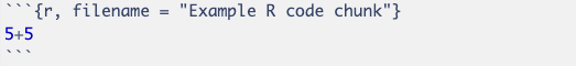
The three backticks (```) mark the beginning of a code chunk, while {r} specifies that the chunk contains R code. To properly close the code chunk, another set of three backticks (```) must be included at the end.

The code inside this chunk is executed, and its results are included in the document below the chunk.

Compiling the Document: knit

To compile the document into your desired output format, click the Knit button in RStudio. This will execute all R code within the document and render it to the specified output format.

Dynamic Report Generation

Knitr allows for the automatic generation of reports. Code chunks embedded within an R Markdown document are executed during the compilation of the document, ensuring that the results (including figures and tables) are directly integrated into the final output.

Multiple Output Formats

With Knitr and R Markdown, you can create a wide range of output formats including HTML, PDF, and Word documents. This flexibility makes it easy to produce reports tailored to different audiences and purposes.

Reproducibility

By combining explanations, source code, and results, documents created with Knitr are not just reports, but also reproducible records of your analysis. This is crucial in scientific research and data analysis where reproducibility is a key concern.

Ease of Use

Knitr uses simple syntax to embed R code in Markdown documents. Code chunks are clearly marked and can be configured with various options to control their behavior and appearance in the output document.

3.4.4 Example: Data Analysis

Here’s a simple example of an R Markdown document that performs a basic data analysis:

Code

Summary of the speed variable in the cars dataset

summary(cars$speed)

   Min. 1st Qu.  Median    Mean 3rd Qu.    Max.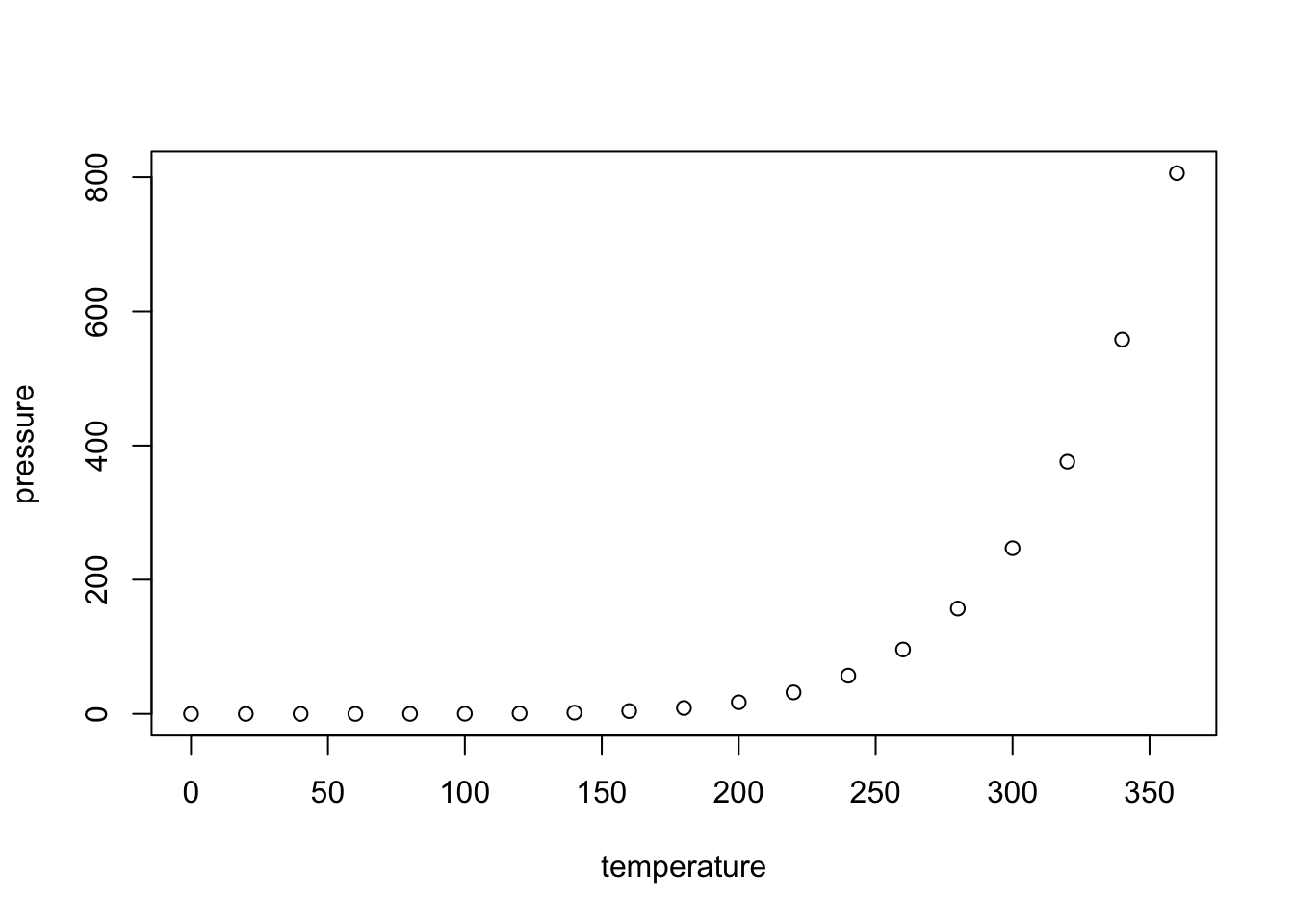 
    4.0    12.0    15.0    15.4    19.0    25.0

Summary Statistics

Let’s calculate summary statistics for the pressure dataset:

Code

summary-stats

summary(pressure)

  temperature     pressure       
 Min.   :  0   Min.   :  0.0002  
 1st Qu.: 90   1st Qu.:  0.1800  
 Median :180   Median :  8.8000  
 Mean   :180   Mean   :124.3367  
 3rd Qu.:270   3rd Qu.:126.5000  
 Max.   :360   Max.   :806.0000

Including Plots

You can also embed plots. For example, here’s a plot of pressure vs temperature:

Code

pressure-plot

plot(pressure)

3.4.5 Chunk options

The most important set of options controls if your code block is executed and what results are inserted in the finished report:

eval = FALSE prevents code from being evaluated. (And obviously if the code is not run, no results will be generated). This is useful for displaying example code, or for disabling a large block of code without commenting each line.
include = FALSE runs the code, but doesn’t show the code or results in the final document. Use this for setup code that you don’t want cluttering your report.
echo = FALSE prevents code, but not the results from appearing in the finished file. Use this when writing reports aimed at people who don’t want to see the underlying R code.
message = FALSE or warning = FALSE prevents messages or warnings from appearing in the finished file.
error = TRUE causes the render to continue even if code returns an error.

Option	Run code	Show code	Output	Plots	Messages	Warnings
`eval = FALSE`
`include = FALSE`	✓
`echo = FALSE`	✓		✓	✓	✓	✓
`results = "hide"`	✓	✓		✓	✓	✓
`fig.show = "hide"`	✓	✓	✓		✓	✓
`message = FALSE`	✓	✓	✓	✓		✓
`warning = FALSE`	✓	✓	✓	✓	✓

3.4.6 PDF Reports: Install tinytex package

To create PDF documents from R Markdown, you will need to have a LaTeX distribution installed. Although there are several traditional options, I recommend that R Markdown users install tinyteX.

Code

Install tinytex package

tinytex::install_tinytex(force = TRUE)

To learn more about R Markdown, Check this ebook

3.4.7 Sample RMarkdown file

3.5 Directories and Projects in R

3.5.1 Introduction

A directory in R is a folder in the computer where files are stored and accessed. R allows users to interact with directories to read data files, save outputs, and manage projects efficiently. Understanding how to check and change the working directory is crucial when dealing with file operations in R.

What is a Working Directory?

The working directory is the default location where R reads and writes files. When working with data files such as CSV, Excel, or text files, R looks for these files in the current working directory unless a full file path is specified.

3.5.2 Setting a New Working Directory:

The setwd() function allows users to change the working directory. This is useful when dealing with files located in different folders.

Syntax:

Code

setwd("/Users/vijay/Library/")

After setting a new directory, you can verify it by running getwd().

Checking the Current Working Directory:

The getwd() function in R is used to check the current working directory. This helps users confirm where R is looking for files and where outputs will be saved.

Syntax:

Code

# Get the current working directory
getwd()

[1] "/Users/vijay/Library/CloudStorage/OneDrive-Personal/Documents/1 Professional/3 My Books/BAAGR"

[1] "/Users/vijay/Library/"

Listing Files in the Current Directory

To check the available files in the current working directory, use list.files():

Code

# List all files in the current working directory
list.files()

This is helpful when verifying whether the required files exist before attempting to read them.

Best Practices for Using Directories in R

Always check the working directory with getwd() before reading or saving files.
Use setwd() cautiously to avoid breaking file paths when sharing scripts across different systems.
Consider using relative paths instead of absolute paths when working on projects in RStudio.

3.6 Overview of Key R Packages

R provides a vast ecosystem of packages designed for data analysis, visualization, and statistical modeling. In this section, we will explore five essential packages:

stats: Statistical analysis and hypothesis testing
plotly: Interactive visualizations
tidyverse: A collection of packages for data manipulation and visualization

Each of these packages serves a crucial role in handling data efficiently and performing complex analyses in R.

3.6.1 stats: Statistical Analysis and Hypothesis Testing in R

The stats package comes pre-installed with R and provides essential statistical functions for data analysis.

Key Features:

Performs descriptive statistics (mean, median, standard deviation).
Supports hypothesis testing (t-tests, ANOVA, chi-square).
Includes regression and time-series analysis.

Basic Usage:

Code

# Descriptive statistics
summary(mtcars$mpg)

   Min. 1st Qu.  Median    Mean 3rd Qu.    Max. 
  10.40   15.43   19.20   20.09   22.80   33.90

Code

# t-test example
t.test(mtcars$mpg ~ mtcars$am)


    Welch Two Sample t-test

data:  mtcars$mpg by mtcars$am
t = -3.7671, df = 18.332, p-value = 0.001374
alternative hypothesis: true difference in means between group 0 and group 1 is not equal to 0
95 percent confidence interval:
 -11.280194  -3.209684
sample estimates:
mean in group 0 mean in group 1 
       17.14737        24.39231

Code

# Linear regression
model <- lm(mpg ~ wt, data = mtcars)
summary(model)


Call:
lm(formula = mpg ~ wt, data = mtcars)

Residuals:
    Min      1Q  Median      3Q     Max 
-4.5432 -2.3647 -0.1252  1.4096  6.8727 

Coefficients:
            Estimate Std. Error t value Pr(>|t|)    
(Intercept)  37.2851     1.8776  19.858  < 2e-16 ***
wt           -5.3445     0.5591  -9.559 1.29e-10 ***
---
Signif. codes:  0 '***' 0.001 '**' 0.01 '*' 0.05 '.' 0.1 ' ' 1

Residual standard error: 3.046 on 30 degrees of freedom
Multiple R-squared:  0.7528,    Adjusted R-squared:  0.7446 
F-statistic: 91.38 on 1 and 30 DF,  p-value: 1.294e-10

3.6.2 plotly: Creating Interactive Visualizations in R

The plotly package enables the creation of interactive and dynamic charts in R, making it useful for exploring data visually.

Key Features:

Supports interactive plots such as scatter plots, bar charts, and 3D plots.
Allows zooming, panning, and tooltips.
Integrates seamlessly with ggplot2.

Basic Usage:

Code

# Install and load the package
install.packages("plotly")

Code

library(plotly)

# Create a simple scatter plot
plot_ly(data = mtcars, x = ~wt, y = ~mpg, type = "scatter", mode = "markers")

Example Use Case:

An agribusiness analyst visualizes seasonal trends in crop yields using plotly, making it easier to identify patterns and variations.

3.6.3 Tidyverse: A Unified Collection of R Packages for Data Science

The tidyverse is a collection of R packages designed for data science. It provides a structured approach to importing, manipulating, visualizing, and modeling data.

Installing and Loading Tidyverse

Code

# Install tidyverse
install.packages("tidyverse")

# Load all core tidyverse packages
library(tidyverse)

This loads several useful packages such as ggplot2, dplyr, tidyr, readr, purrr, tibble, stringr, and forcats.

3.6.4 Key Functionalities of Tidyverse

1. Data Manipulation with dplyr

Code

library(dplyr)

# Sample dataset
data <- tibble(Name = c("John", "Alice", "Bob"), Score = c(85, 90, 78))

# Filtering rows where Score > 80
filtered_data <- data %>% filter(Score > 80)

# Summarizing average score
average_score <- data %>% summarize(Avg_Score = mean(Score))

print(filtered_data)

# A tibble: 2 × 2
  Name  Score
  <chr> <dbl>
1 John     85
2 Alice    90

Code

print(average_score)

# A tibble: 1 × 1
  Avg_Score
      <dbl>
1      84.3

2. Data Tidying with tidyr

Code

library(tidyr)

# Sample dataset (wide format)
data <- tibble(Name = c("A", "B"), Math = c(85, 90), Science = c(78, 92))

# Convert to long format
long_data <- pivot_longer(data, cols = c(Math, Science), names_to = "Subject", values_to = "Marks")

print(long_data)

# A tibble: 4 × 3
  Name  Subject Marks
  <chr> <chr>   <dbl>
1 A     Math       85
2 A     Science    78
3 B     Math       90
4 B     Science    92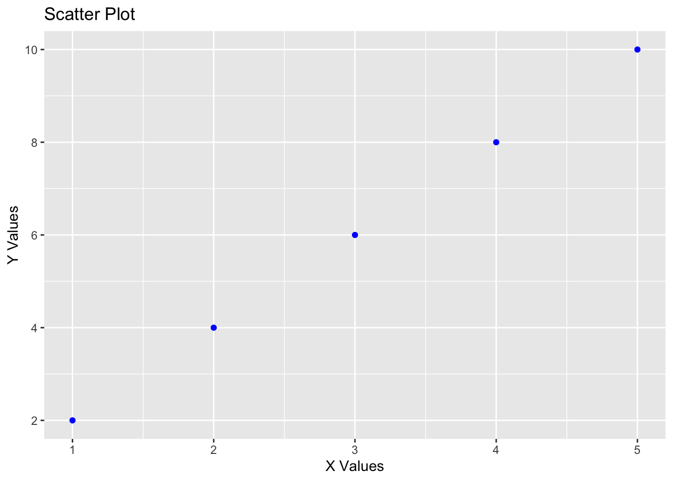

3. Data Visualization with ggplot2

Code

library(ggplot2)

# Sample dataset
data <- tibble(x = c(1, 2, 3, 4, 5), y = c(2, 4, 6, 8, 10))

# Create a scatter plot
ggplot(data, aes(x = x, y = y)) +
  geom_point(color = "blue") +
  labs(title = "Scatter Plot", x = "X Values", y = "Y Values")

4. String Manipulation with stringr

Code

library(stringr)

text <- "Welcome to R programming!"

# Convert to lowercase
lower_text <- str_to_lower(text)

# Replace "R" with "Tidyverse"
new_text <- str_replace(text, "R", "Tidyverse")

print(lower_text)

[1] "welcome to r programming!"

Code

print(new_text)

[1] "Welcome to Tidyverse programming!"

5. Handling Factors with forcats

Code

library(forcats)

# Sample categorical data
fruit <- factor(c("Apple", "Banana", "Cherry", "Banana", "Apple"))

# Reorder factor levels based on frequency
reordered_fruit <- fct_infreq(fruit)

print(reordered_fruit)

[1] Apple  Banana Cherry Banana Apple 
Levels: Apple Banana Cherry