[1] 20Code
sample_mean = mean(scores)
sample_mean
[1] 76.85Population and Sample
Parameter and Statistic
Standard deviation of population:
The formula for the standard deviation of a population (\(s\)) is:
\[ \sigma = \sqrt{\frac{1}{n} \sum_{i=1}^{n} (x_i - \mu)^2} \]
where:
Standard deviation of sample:
The formula for the standard deviation of a sample (\(s\)) is:
\[ s = \sqrt{\frac{1}{n-1} \sum_{i=1}^{n} (x_i - \bar{x})^2} \]
where:
The formula for the sample standard deviation (\(\sigma\)) is similar but divides by \(n-1\) instead of \(n\):
The divisor \(n-1\) in the sample standard deviation formula accounts for the degrees of freedom in the estimation of the standard deviation and corrects the bias in the estimation of the population standard deviation from a sample. This correction is known as Bessel’s correction.
Sample Standard Deviation
[1] 9.371148Population Standard Deviation
Sample Standard Deviation
python
import numpy as np
scores= np.array([66,84,70,72,73,86,75,88,62,81,85,63,79,79,83,90,61,82,69,89])
sample_size =len(scores)
sample_size20# Calculate sample mean
sample_mean = np.mean(scores)
sample_mean76.85python
# Calculate the standard deviation for the sample
# The default ddof=1 is used for sample standard deviation
sample_sd= np.std(scores, ddof=1)
sample_sd9.371148331588376Population Standard Deviation
python
# Calculate the standard deviation for the population
# The default ddof=0 is used for population standard deviation
population_sd = np.std(scores, ddof=0)
population_sd9.133865556269154download the dataset here
R
library(readxl)
# laod data and View
data_bank <- read_excel("Bank Customer Churn Prediction.xlsx")
data_bank
# A tibble: 10,000 × 12
customer_id credit_score country gender age tenure balance products_number
<dbl> <dbl> <chr> <chr> <dbl> <dbl> <dbl> <dbl>
1 15634602 619 France Female 42 2 0 1
2 15647311 608 Spain Female 41 1 83808. 1
3 15619304 502 France Female 42 8 159661. 3
4 15701354 699 France Female 39 1 0 2
5 15737888 850 Spain Female 43 2 125511. 1
6 15574012 645 Spain Male 44 8 113756. 2
7 15592531 822 France Male 50 7 0 2
8 15656148 376 Germany Female 29 4 115047. 4
9 15792365 501 France Male 44 4 142051. 2
10 15592389 684 France Male 27 2 134604. 1
# ℹ 9,990 more rows
# ℹ 4 more variables: credit_card <dbl>, active_member <dbl>,
# estimated_salary <dbl>, churn <dbl>sample_size <- length(data_bank$credit_score)
sample_size[1] 10000# Calculate sample mean
sample_mean <- mean(data_bank$credit_score)
sample_mean[1] 650.5288# Calculate sample standard deviation
sample_sd <- sd(data_bank$credit_score)
sample_sd[1] 96.6533[1] 96.64847To load excel data into python, install openpyxl in jupyter notebook using the command !pip3 install pandas openpyxl
python
import pandas as pd
import numpy as np
# Load data
data_bank = pd.read_excel("Bank Customer Churn Prediction.xlsx")
data_bank
customer_id credit_score ... estimated_salary churn
0 15634602 619 ... 101348.88 1
1 15647311 608 ... 112542.58 0
2 15619304 502 ... 113931.57 1
3 15701354 699 ... 93826.63 0
4 15737888 850 ... 79084.10 0
... ... ... ... ... ...
9995 15606229 771 ... 96270.64 0
9996 15569892 516 ... 101699.77 0
9997 15584532 709 ... 42085.58 1
9998 15682355 772 ... 92888.52 1
9999 15628319 792 ... 38190.78 0
[10000 rows x 12 columns]# Calculate sample mean of credit score
sample_mean = np.mean(data_bank['credit_score'])
sample_mean650.5288# Calculate sample standard deviation of credit score
sample_sd = np.std(data_bank['credit_score'], ddof=1)
sample_sd96.65329873613035# Calculate population standard deviation of credit score
population_sd = np.std(data_bank['credit_score'], ddof=0)
population_sd96.64846595037089Hypothesis testing is a statistical method used to make decisions about a population based on sample data. It’s a core concept in statistics and research, allowing scientists, analysts, and decision-makers to test assumptions, theories, or hypotheses about a parameter (e.g., mean, proportion) of a population.
Hypotheses: In hypothesis testing, two opposing hypotheses are formulated:
Significance Level (\(\alpha\)): It’s the threshold for rejecting the null hypothesis, typically set at 0.05 (5%). It represents the probability of rejecting the null hypothesis when it’s actually true, known as Type I error.
P-value: The probability of observing the sample data, or something more extreme, if the null hypothesis is true. A small p-value (typically ≤ 0.05) indicates strong evidence against the null hypothesis.
Test Statistic: A value calculated from the sample data, used to evaluate the likelihood of the null hypothesis. The form of the test statistic depends on the test type (e.g., z-test, t-test).
Formulate Hypotheses: Define the null and alternative hypotheses based on the research question.
Choose the Significance Level: Set the \(\alpha\) level (e.g., 0.05).
Select the Appropriate Test: Based on the data type and hypothesis, choose a statistical test (e.g., t-test for comparing means).
Calculate the Test Statistic: Use the sample data to compute the test statistic.
Determine the P-value: Find the probability of observing the test results under the null hypothesis.
Make a Decision: Compare the p-value to \(\alpha\). If the p-value is less than \(\alpha\), reject the null hypothesis; otherwise, fail to reject it.
Most statistical tests have underlying assumptions about the data (e.g., normality, independence, homoscedasticity). Violating these assumptions can affect the validity of the test results.
- It’s important to choose the right test based on these assumptions or use non-parametric tests that don’t rely on such assumptions.
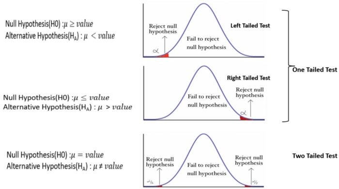
A hypothesis test can be one-tailed or two-tailed, depending on the nature of the alternative hypothesis.
One-tailed and two-tailed tests are two approaches to statistical hypothesis testing that are used to determine if there is enough evidence to reject the null hypothesis, considering the directionality of the relationships or differences.
A one-tailed test, also known as a directional test, is used when the research hypothesis specifies the direction of the relationship or difference. It tests for the possibility of the relationship in one specific direction and ignores the possibility of a relationship in the other direction. This makes a one-tailed test more powerful than a two-tailed test for detecting an effect in one direction because all the statistical power of the test is focused on detecting an effect in that one direction.
When to use: - If you have a specific hypothesis that states one variable is greater than or less than the other variable. - If the consequences of missing an effect in one direction are not as critical as in the other direction.
Example: Suppose you are testing a new drug and believe that it will be more effective than the current treatment. You would use a one-tailed test to determine if the new drug is significantly better.
A two-tailed test, or a non-directional test, is used when the research hypothesis does not specify the direction of the expected relationship or difference. It tests for the possibility of the relationship in both directions. This means that it checks for both, whether one variable is either greater than or less than the other variable, thus requiring more evidence to reject the null hypothesis compared to the one-tailed test.
When to use: - If you do not have a specific direction in mind or if you are interested in detecting any significant difference, regardless of the direction. - If the consequences of missing an effect are equally important in both directions.
Example: Suppose you are testing a new teaching method and want to find out if it has a different effect (either better or worse) on students’ test scores compared to the traditional method. A two-tailed test would be appropriate in this case.
The choice between a one-tailed and two-tailed test should be determined by the research question or hypothesis. One-tailed tests are more powerful for detecting an effect in one direction but at the cost of potentially missing an effect in the other direction. Two-tailed tests are more conservative and are used when it is important to detect effects in either direction.
Considerations: