29 Understanding the Machine Learning Analytical Cycle
Building a machine learning model is never a single step. It’s a cycle of well-defined phases, from framing the problem through to watching the deployed model over time. This topic walks through that cycle twice, from two complementary angles: Architecture follows the cycle as a sequence of steps, in the order a project actually moves through them, using one running example, predicting crop yield from rainfall, fertilizer use, and soil conditions. Key Components then steps back and looks at the same cycle as a set of reusable building blocks, the layers a data team maintains across many projects, not just one.
29.1 Basic Architecture of the Analytical Cycle in Machine Learning
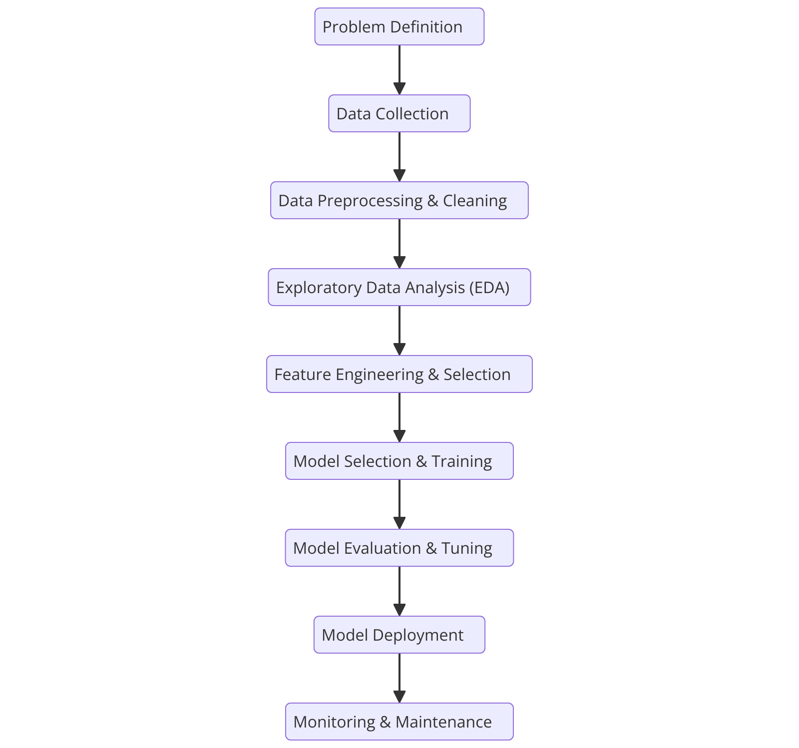
The machine learning analytical cycle consists of multiple interconnected phases, each playing a vital role in ensuring that data is used effectively to build accurate predictive models (Rüdiger Wirth & Jochen Hipp, 2000). The worked example below follows all nine steps for one concrete problem: predicting a farm’s crop yield (tons/hectare) from rainfall, fertilizer use, and soil moisture.
Step 1: Problem Definition
- Clearly define the business or research problem that needs to be addressed.
- Determine the type of ML model (supervised, unsupervised, reinforcement learning) required.
- Example: an agribusiness cooperative wants to predict a farm’s crop yield ahead of harvest, so it can plan storage and logistics. This is a supervised regression problem. The target (yield) is a known numeric outcome in historical data.
Step 2: Data Collection
- Gather relevant raw data from multiple sources. Weather stations, soil sensors, farm records, satellite imagery, procurement logs.
- Ensure data relevance, quality, and availability for training the model.
- Example: collecting each farm’s seasonal rainfall totals, fertilizer application records, soil-moisture readings, and the resulting harvest yield for the past several seasons.
Step 3: Data Preprocessing & Cleaning
- Handle missing values, duplicates, and outliers (see Data Import and Cleaning).
- Convert categorical variables into numerical form (dummy encoding, label encoding. See Creating and Managing Dummy Variables).
- Normalize or standardize data to bring variables onto a common scale (see Normalization and Standardization).
- Example: filling a handful of missing fertilizer readings, removing a duplicated farm record, and encoding irrigation type as a dummy variable.
Step 4: Exploratory Data Analysis (EDA)
- Use statistical methods and visualization tools to understand patterns, trends, and correlations (see Scatter Plot and Histogram).
- Identify which variables appear to influence the outcome.
- Example: a scatter plot of rainfall against yield suggests a positive relationship; a box plot of yield by irrigation type shows canal-irrigated farms out-yielding rainfed ones (see Box Plots).
Step 5: Feature Engineering & Selection
- Transform raw data into meaningful features that improve model performance.
- Apply feature selection techniques (filter, wrapper, or embedded methods) to remove redundant features.
- Example: combining rainfall and irrigation records into a single “effective water supply” feature, rather than feeding the model two overlapping raw variables.
Step 6: Model Selection & Training
- Choose the appropriate machine learning algorithm (e.g., linear regression, decision trees, random forests) for the problem type.
- Split data into training and testing sets (e.g., an 80/20 split) so the model’s performance can be checked on data it hasn’t seen.
- Train the model on the training set.
- Example: training a regression model to predict yield from rainfall, fertilizer, and soil moisture.
Step 7: Model Evaluation & Tuning
- Use evaluation metrics (RMSE, MAE, R² for regression; accuracy, precision, recall, F1-score for classification) to measure model performance on the held-out test set.
- Perform hyperparameter tuning (grid search, random search) to improve the model.
- Example: checking how far off the model’s yield predictions are, on average, from farms it wasn’t trained on.
Step 8: Model Deployment
- Put the trained model into a real-world environment, a web app, an API, a dashboard the cooperative’s agronomists can use.
- Integrate it with existing business processes and monitor how it performs in practice.
- Example: making the yield model available through a simple dashboard the cooperative’s field staff check ahead of each harvest.
Step 9: Monitoring & Maintenance
- Continuously track model performance to detect drift. A model trained on three normal seasons can degrade sharply after an unusual drought or flood year.
- Retrain periodically with new data to keep predictions accurate.
- Example: re-checking the yield model’s accuracy each season and retraining it once enough new harvest data has come in.
29.1.1 A Worked Example in R: Steps 6–7 in Practice
The example below runs Steps 6 and 7 end to end on a small farm dataset: split the data, train a simple regression model, and evaluate it on data the model hasn’t seen.

RMSE and MAE report the average prediction error in the same units as yield (tons/ha). Smaller is better. R² reports how much of the variation in test-set yield the model explains. Closer to 1 is better. A model with a small RMSE and a high R² on data it never saw during training is one worth deploying; a model that fits the training data well but performs poorly here is overfit, and needs revisiting at Step 5 or 6 before it goes anywhere near Step 8.
29.2 Key Components of an Analytical Process
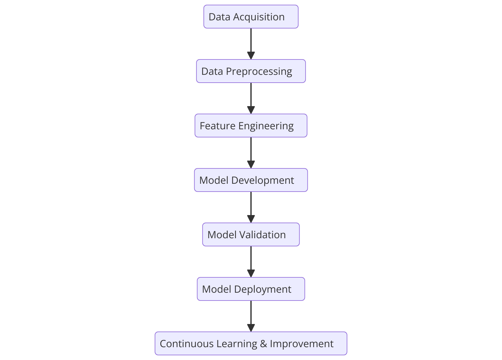
The nine steps above describe one project’s path through the cycle, start to finish. Zoom out, and a data team maintains the same handful of layers across every project it runs, not a one-time sequence, but ongoing responsibilities. Framed this way, the analytical process breaks into six components:
1. Data Layer
- The pipelines and storage that keep raw data flowing in reliably. Weather-station feeds, farm-record uploads, satellite imagery archives.
- Owned by whoever maintains data collection and quality, independent of any one model.
2. Preparation Layer
- The reusable cleaning and transformation logic (handling missing sensor readings, standardizing units across data sources) that every new project draws on rather than rebuilding.
3. Feature Layer
- A shared library of engineered features (“effective water supply,” “growing-degree days,” “days since last fertilizer application”) that multiple models across the organization can reuse.
4. Modeling Layer
- The set of algorithms and training infrastructure available to a project (from a simple regression to a random forest or neural network) plus the compute needed to train them at scale.
- Example: a shared modeling environment used for both the yield-prediction project and a separate pest-outbreak-risk project.
5. Evaluation & Validation Layer
- Standard metrics and testing practices (train/test splits, cross-validation, agreed-upon metrics) applied consistently so models across different projects can be compared fairly.
- Example: every predictive model the cooperative builds is evaluated on RMSE and R² using the same held-out-season convention, so a yield model and a price-forecasting model are judged the same way.
6. Deployment & Monitoring Layer
- The infrastructure that serves model predictions to users and watches for drift over time: dashboards, APIs, alerting when accuracy drops.
- Example: the same monitoring dashboard that tracks the yield model’s seasonal accuracy could also host a crop-disease-risk model built later, without rebuilding the monitoring layer from scratch.
Where the nine-step architecture answers “what do we do, in order, to ship this model?”, the six components answer “what do we need to keep working, on an ongoing basis, to ship many models?” A single small project might treat all six as one person’s job; a larger analytics team typically has different people, or even different tools, responsible for each layer.
Summary
| Concept | Description |
|---|---|
| Basic Architecture of the Analytical Cycle in Machine Learning | |
| Step 1: Problem Definition | Frame the business or research problem and decide the type of ML task, e.g., predicting crop yield as a supervised regression problem |
| Step 2: Data Collection | Gather relevant raw data from weather stations, sensors, farm records, and other sources |
| Step 3: Data Preprocessing & Cleaning | Clean missing values and duplicates, encode categorical variables, and normalize or standardize numeric variables |
| Step 4: Exploratory Data Analysis (EDA) | Use statistics and visualization to understand patterns, trends, and correlations in the data |
| Step 5: Feature Engineering & Selection | Transform raw data into meaningful features and remove redundant ones |
| Step 6: Model Selection & Training | Choose an algorithm, split data into training and testing sets, and train the model |
| Step 7: Model Evaluation & Tuning | Evaluate the trained model on held-out data using metrics like RMSE, MAE, R-squared, or accuracy, and tune hyperparameters |
| Step 8: Model Deployment | Put the trained model into a real-world environment such as a dashboard or API |
| Step 9: Monitoring & Maintenance | Track the deployed model's performance over time and retrain as new data arrives |
| Key Components of an Analytical Process | |
| Data Layer | The pipelines and storage that keep raw data flowing in reliably across projects |
| Preparation Layer | Reusable cleaning and transformation logic shared across projects |
| Feature Layer | A shared library of engineered features multiple models can reuse |
| Modeling Layer | The algorithms and training infrastructure available for building models |
| Evaluation & Validation Layer | Standard metrics and testing practices applied consistently across models |
| Deployment & Monitoring Layer | The infrastructure that serves predictions and monitors deployed models for drift |