38 T-Tests
The t-test (Student, 1908) is a foundational statistical hypothesis test used to determine whether there is a significant difference between the means of two groups, or between a single group’s mean and a known or claimed value.
- It is applied when the test statistic would follow a normal distribution if a scaling term in the test statistic were known, but that term instead has to be estimated from the sample.
- Because the scaling term (the population standard deviation) is estimated rather than known, the test statistic follows a Student’s t-distribution rather than the normal distribution.
38.0.1 When to Use a T-Test
- Small samples: the t-test extends the logic of a Z-test to situations where the sample size is small (usually \(n < 30\)) and the population variance is unknown.
- Student’s t-distribution: the t-test uses the t-distribution, which is more spread out than the normal (Z) distribution, especially for small sample sizes. Its exact shape depends on the degrees of freedom. A concept the Z-test doesn’t need.
38.0.2 Degrees of Freedom
Degrees of freedom (df) refers to the number of values in a calculation that are free to vary once certain constraints (like a sample mean already being fixed) are imposed.
- A t-test uses the sample standard deviation as an estimate of the population standard deviation. That estimation introduces extra uncertainty, which is why the wider, thicker-tailed t-distribution is used instead of the normal distribution.
- By contrast, a Z-test uses the population standard deviation (\(\sigma\)) directly, which is assumed to be known. Because nothing is estimated from the sample, no degrees-of-freedom correction is needed, and the test statistic follows the standard normal (Z) distribution regardless of sample size.
Degrees of freedom differ by t-test type:
| T-Test Type | Degrees of Freedom |
|---|---|
| One-sample | \(n - 1\) |
| Independent two-sample (pooled) | \(n_1 + n_2 - 2\) |
| Paired | \(n - 1\) (number of pairs minus one) |
38.0.3 Types of T-Tests
One-sample t-test: compares the mean of a single group against a known or claimed value, for example, checking whether the average yield of a hybrid seed variety matches the seed company’s claim.
Independent samples t-test: compares the means of two independent groups to see whether their population means differ, for example, comparing yields between two different seed varieties grown on separate plots.
Paired samples t-test: compares the means of the same group measured under two conditions or at two points in time, for example, measuring the same plots’ yield before and after switching to a new fertilizer program.
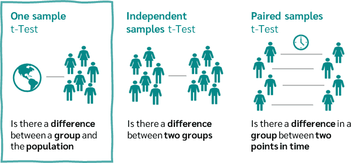
source: https://datatab.net/tutorial/one-sample-t-test
38.0.4 Assumptions
- Independence: observations must be independent of one another.
- Normality: the data should be approximately normally distributed, which matters less as sample size grows (Central Limit Theorem).
- Equality of variances (for the independent-samples t-test only): classically assumed equal; when it doesn’t hold, Welch’s t-test is used instead. R’s
t.test()actually defaults to Welch’s t-test rather than assuming equal variances. See the independent-samples example below.
38.0.5 Interpretation and Effect Size
A t-test’s p-value indicates how likely the observed result (or something more extreme) would be if the null hypothesis were true. If the p-value is below the chosen significance level (commonly 0.05), the null hypothesis is rejected.
A p-value alone doesn’t say how large the difference is. For that, report Cohen’s d, a standardized effect size:
\[d = \frac{\bar{x} - \mu_0}{s} \quad \text{(one-sample)} \qquad d = \frac{\bar{X}_1 - \bar{X}_2}{s_p} \quad \text{(two-sample, pooled SD)}\]
By convention, \(|d| \approx 0.2\) is a small effect, \(0.5\) medium, and \(0.8\) large. It’s good practice to report a confidence interval for the mean or mean difference alongside the p-value. R’s t.test() output includes one automatically.
38.1 One-Sample T-Test
The one-sample t-test determines whether the mean of a single sample differs significantly from a known or hypothesized value. It’s useful when the population standard deviation is unknown and the sample size is small.
Assumptions
- Normality: the data should be approximately normally distributed, especially with a small sample.
- Independence: observations must be independent of each other.
- Scale of measurement: the data should be at least interval-scaled.
Formula
\[t = \frac{\bar{x} - \mu_0}{s / \sqrt{n}}, \qquad df = n - 1\]
Where \(\bar{x}\) is the sample mean, \(\mu_0\) is the hypothesized value, \(s\) is the sample standard deviation, and \(n\) is the sample size.
Example: Does a Hybrid Maize Variety Meet Its Claimed Yield?
A seed company claims its hybrid maize variety yields at least 60 quintals per hectare on average. An agricultural extension officer is skeptical and samples 15 plots that grew the variety, recording yield (quintals/hectare) on each:
52, 55, 61, 54, 58, 59, 62, 53, 56, 57, 60, 59, 61, 64, 58Because the claim itself is one-directional (“at least 60”), the natural test is one-tailed: is the true mean yield actually less than 60? The officer chooses a significance level of 0.05.
Hypotheses
- Null Hypothesis (\(H_0\)): \(\mu \geq 60\). The mean yield meets or exceeds the claim.
- Alternative Hypothesis (\(H_1\)): \(\mu < 60\). The mean yield falls short of the claim.
This is a one-tailed (lower-tail) test, since only a shortfall would contradict the claim; a yield well above 60 would never make the officer reject the seed company’s claim.
Sample Mean and Standard Deviation
The sample size \(n\) is 15.
\[\bar{x} = \frac{52 + 55 + 61 + 54 + 58 + 59 + 62 + 53 + 56 + 57 + 60 + 59 + 61 + 64 + 58}{15} = \frac{869}{15} = 57.93 \text{ quintals/hectare}\]
\[s = \sqrt{\frac{\sum (x_i - \bar{x})^2}{n-1}} = \sqrt{\frac{167.07}{14}} = 3.45 \text{ quintals/hectare}\]
T-Statistic, Degrees of Freedom, and P-Value
\[t = \frac{\bar{x} - \mu_0}{s / \sqrt{n}} = \frac{57.93 - 60}{3.45 / \sqrt{15}} = -2.32, \qquad df = 15 - 1 = 14\]
For a one-tailed test, the p-value is the area to the left of \(t = -2.32\) under the t-distribution with 14 df: \(p \approx 0.018\).
Cohen’s d: \(d = \dfrac{57.93 - 60}{3.45} \approx -0.60\), a medium-to-large effect.
95% confidence interval for the mean: approximately \([56.02,\ 59.85]\) quintals/hectare. Notice the interval sits entirely below 60, consistent with rejecting the claim.
Interpretation
- The p-value (0.018) is below \(\alpha = 0.05\), so the null hypothesis is rejected.
- There is statistically significant evidence that the hybrid maize variety’s true mean yield is below the company’s claimed 60 quintals/hectare, by a medium-to-large margin (Cohen’s \(d \approx -0.60\)), not just a statistically detectable but trivial one.
One-Sample T-Test in R

38.2 Independent Samples T-Test (Two-Sample T-Test)
The independent (two-sample) t-test determines whether there is a significant difference between the means of two independent groups, for instance, two seed varieties grown on separate, unrelated plots.
Assumptions
- Independence: the two groups must be independent, the plots for one variety don’t influence the plots for the other.
- Normality: yield in each group should be roughly normally distributed.
- Equality of variances: classically assumed; if violated, Welch’s t-test is the safer default. R’s
t.test()uses Welch’s t-test unlessvar.equal = TRUEis explicitly requested, the worked example below uses this current default rather than forcing equal variances.
Formula
\[t = \frac{\bar{X}_1 - \bar{X}_2}{s_p \sqrt{\dfrac{1}{n_1} + \dfrac{1}{n_2}}}, \qquad s_p = \sqrt{\frac{(n_1-1)s_1^2 + (n_2-1)s_2^2}{n_1+n_2-2}}, \qquad df = n_1 + n_2 - 2\]
This is the classical pooled-variance formula. Welch’s t-test, R’s default, adjusts the standard error and degrees of freedom to account for possibly unequal variances instead of pooling them. For data this close in spread, the two approaches give nearly identical results, as the worked example shows.
Example: Comparing Yield Between Two Seed Varieties
An agronomist wants to know whether two seed varieties differ in yield (quintals/acre). Five plots were sown with each variety:
- Variety P: 85, 88, 90, 95, 78
- Variety Q: 80, 83, 79, 92, 87
We test at \(\alpha = 0.05\).
Hypotheses
- Null Hypothesis (\(H_0\)): \(\mu_P = \mu_Q\)
- Alternative Hypothesis (\(H_1\)): \(\mu_P \neq \mu_Q\)
Calculation (Pooled-Variance Method)
\[\bar{X}_P = \frac{85+88+90+95+78}{5} = 87.2, \qquad \bar{X}_Q = \frac{80+83+79+92+87}{5} = 84.2\]
\[s_P^2 = \frac{(-2.2)^2+(0.8)^2+(2.8)^2+(7.8)^2+(-9.2)^2}{4} = 39.7, \qquad s_Q^2 = \frac{(-4.2)^2+(-1.2)^2+(-5.2)^2+(7.8)^2+(2.8)^2}{4} = 28.7\]
\[s_p^2 = \frac{(4)(39.7) + (4)(28.7)}{8} = 34.2\]
\[t = \frac{87.2 - 84.2}{\sqrt{34.2}\sqrt{\tfrac{1}{5}+\tfrac{1}{5}}} = \frac{3}{5.85 \times 0.632} \approx 0.811, \qquad df = 5+5-2 = 8\]
For \(df = 8\), the two-tailed critical value at \(\alpha = 0.05\) is 2.306. Since \(|0.811| < 2.306\), we fail to reject \(H_0\) (\(p \approx 0.44\)).
Cohen’s d: \(d = \dfrac{87.2-84.2}{\sqrt{34.2}} \approx 0.51\), a medium effect in raw terms, even though it isn’t statistically significant with only 5 plots per group. That gap is a useful reminder: a non-significant result with a small sample doesn’t prove there’s no real difference, only that this sample couldn’t detect one confidently.
Independent Samples T-Test in R
38.3 Paired Samples T-Test
The paired (dependent) samples t-test compares two related sets of measurements, typically the same subjects measured twice, such as the same plots’ yield before and after an intervention.
Key Applications
- Comparing before-and-after effects of an intervention on the same plots or farms.
- Measuring the same subjects under two different conditions.
- Crossover studies, where the same subjects receive both treatments.
Assumptions
- Paired data: observations come as matched pairs (same plots, before/after).
- Normality of differences: the differences between pairs should be roughly normally distributed.
- Scale of measurement: at least interval-scaled data.
Formulae
\[\bar{d} = \frac{1}{n}\sum_{i=1}^{n}(x_{i1}-x_{i2}), \qquad s_d = \sqrt{\frac{\sum(d_i-\bar{d})^2}{n-1}}, \qquad t = \frac{\bar{d}}{s_d/\sqrt{n}}, \qquad df = n-1\]
Example: Yield Before and After a New Fertilizer Program
An agronomist tests a new organic fertilizer program on 5 plots, recording yield (quintals/acre) before and 6 weeks after adopting it:
- Before: 70, 72, 75, 80, 78
- After: 68, 70, 74, 77, 76
Wait. Yield actually decreased on every plot here. This is deliberately used as a paired-test example of a negative result: the new program did not improve yield in this trial, and the paired test lets us confirm that the decrease is too consistent to be chance. We test at \(\alpha = 0.05\).
Calculation
\[d = [2, 2, 1, 3, 2] \text{ (Before − After, quintals/acre)}\]
\[\bar{d} = \frac{2+2+1+3+2}{5} = 2, \qquad s_d = \sqrt{\frac{0+0+1+1+0}{4}} = \sqrt{0.5} = 0.707\]
\[t = \frac{2}{0.707/\sqrt{5}} = \frac{2}{0.316} = 6.32, \qquad df = 5-1=4\]
The two-tailed critical value at \(df=4\), \(\alpha=0.05\) is 2.776. Since \(6.32 > 2.776\), we reject \(H_0\) (\(p \approx 0.003\)).
Cohen’s d (paired): \(d = \dfrac{\bar{d}}{s_d} = \dfrac{2}{0.707} \approx 2.83\). A very large effect. 95% CI for the mean difference: approximately \([1.12,\ 2.88]\) quintals/acre, entirely on the “yield dropped” side of zero.
Interpretation
The consistent, statistically significant drop (large Cohen’s d, CI excluding zero) indicates the new fertilizer program was associated with lower yield in this trial, a result worth investigating before wider rollout, not a program to celebrate.